
Background and Project Objective
Recommendation systems are quickly gaining popularity with companies seeking a way to predict user preferences based on past experience. Specifically, these recommendation systems typically aim to maximize the chance that a user will engage with a recommended product. Recommendation tasks appear in a wide range of business contexts, from e-commerce to social networking.
In the scope of this report we present and compare several solutions for the specific challenge of building a production-grade recommendation system using the Yelp Open Dataset from the 2019 challenge.
More precisely, the Yelp Dataset is a vast dataset of business reviews left by users of the Yelp platform. We’ll use this data to develop an array of models that aim to predict the last review of a business for each user in the dataset (on a scale of 1 to 5 stars). To evaluate the performance of our models, we will compare the ratings our models predict against the actual rating the user left for that business. Depending on the business objective, there are a number of ways to define a successful prediction (and a successful model). We present our business objective and model evaluation framework below.
Business Problem and High-Level Objectives
Building an effective recommendation system is challenging because, in addition to requiring a familiarity with algorithmic recommendation techniques, making good predictions depends on business domain knowledge. Knowing the specifics of your product and its users is key to designing and building an effective recommendation system for all subsets of users and businesses in the dataset.
To that end, there is a tremendous variety of users and businesses in the dataset. For example, there are thousands of businesses categories, and each business can fall into several categories. Additionally, we have users with over one thousand reviews, and users with a single review, and these users are scattered across thousands of cities. Intuition suggests that a one-size-fits-all solution will not provide effective recommendations for this variety of users and businesses.
With these diversity considerations in mind, our main business objective is to understand which models work well for various subsets of our users and businesses. That is, if model A performs well for new users, model B performs well for businesses from niche categories, and model C performs well for popular users and items, we can devise a model switching strategy to serve optimal recommendations for as many users as possible.
Of course, this begs the secondary question: what exactly is a “good” recommendation? In this context, we define a good business recommendation for a user as one that has a similar rank (relative to other businesses) as the user’s actual rank for that business. In other words, we hypothesize that we risk losing users if we recommend a business that the user really dislikes, but we can retain a user if a tolerable (even if mediocre) business is recommended. Our “coverage” metric seeks to minimize these terrible recommendations. We will compare models on the basis of this metric.
In summary, aim to segment users and businesses, evaluate the performance of our models with respect to these segments on a meaningful metric, and ultimately propose a model-switching strategy for our business.
Detailed Objectives
The general objective of this project is to design, build and evaluate recommendation models that predict the stars a Yelp user gives to business. More accurately, to predict the stars for the last business the user went, considering only active users (users with 5 or more reviews in the dataset).
Our specific objective, as outlined above, is to evaluate the performance of several models on various subsets of the data, optimizing for “coverage” (defined as avoiding a highly negative recommendation experience for a user). This metric is more meaningful for our business case.
Finally, some of the models we test will incorporate contextual data from business and users in the Yelp dataset, including business categories. From the second half of the semester, we will experiment with the following categories of models: Deep-learning-based recommendation models Content-based recommendation models
Data Exploration
Data Completeness:
The dataset is remarkably complete! Only the following features had a significant number of missing records: Businesses:
- Attributes: 15% missing
- Hours: 23% missing
- Address: 4% missing
Users and Reviews: No missing data!
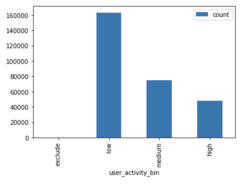
Distribution of users by activity and businesses by popularity:
We segmented both users and businesses into three categories.
Users:
- Exclude = 1-4 reviews
- Low-activity definition: 5-10 reviews
- Medium-activity: 11-20 reviews
- High-activity: 20+ reviews
- Distribution:
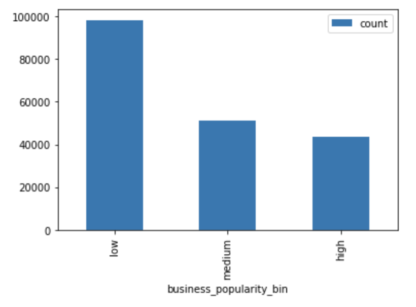
Businesses:
- Low-popularity: 1-10 reviews
- Medium-popularity: 10-30 reviews
- High-popularity: 30+ reviews
- Distribution:
Mean rating across several dimensions:
We computed the mean rating across the following dimensions. The idea is to determine if any single dimension is particularly important when it comes to prediction. If so, we can incorporate this dimension as a feature into any one of our subsequent models:
- City: Montreal and Scottsdale have ratings; Toronto is low.
- State: Similar results to city-cut above.
- Is_open: Unsurprisingly, closed businesses have low ratings.
- Business popularity bin: Unsurprisingly, popular businesses have high ratings (by definition)
- User activity bin: We exclude users with less than 5 ratings, but of the 4 user categories, these users are the most pessimistic.


Recommendation Models
Baseline Models
Before we can determine whether our more advanced recommendation algorithms are successful, we need to establish recommendation benchmarks that we hope to beat. We have three models that will provide baselines for us:
Bias Model
This model serves as our true baseline because it is the most naive approach we attempt. This model works by calculating the global mean (all user-item ratings), and then for each prediction, adding both the mean user and item ratings.
Matrix Factorization Model
We used a model-based collaborative filtering approach. Specifically, we use our PySpark implementation from project #1.
We expect this model to perform relatively well for popular businesses (i.e. those with many reviews) and prolific users (those with many reviews). Presumably, the model will be able to learn the preferences of this group of users by virtue of their high number of interactions, but we expect collaborative filtering to struggle with the cold start problem (users or businesses for which we have few or zero reviews).
Model-Based Collaborative Filtering Model
Additionally, tried a second model-based collaborative filtering technique; specifically singular value decomposition (SVD), for which we used the implementation from the Surprise Python package.
We expect this model to have the same strengths and limitations as our Matrix Factorization model.
Proposed Models
In this project, we aim to outperform our baseline models by trying two new techniques that were presented in the second half of the Fall 2019 semester:
- Deep-learning-based recommendation models
- Content-based recommendation models
Deep Learning Models
By using deep learning models, we hope we can leverage the ability of these models to learn and capture non-linear relationship between the different features of our data, learning and updating weights of these relationships using methods such as gradient descent. Specifically, we propose two types of deep learning models using two types of datasets (different features) from the Yelp dataset.
We used the same architecture for both models, a sequential model mainly composed of dense layer (fully connected neurons layers) and use the mean squared error as the function to optimize the loss of the model:
- layers.Dense(128, activation=’relu’),
- layers.Dense(128, activation=’tanh’),
- layers.Dense(64, activation=’relu’),
- layers.Dense(5, activation=’softmax’)
On top of these layers we provide our features of data as embeddings vectors as input of the model. We track the accuracy and root mean squared error for the training and validation sets while the model trains.
-
Deep Learning Classification approach: we propose a model in which every rating can be seen as a class (from 1 to 5) and so the model learns relationships from the different features of data and predict the probability of each observation to belong to each class. For this type of model to work, we encode each rating as a one-hot vector, so we can have a one-hot vector of probabilities using the activation function ‘softmax’ for the last layer of the model, which give us a vector of probabilities in the space 0-1.
-
Deep Learning Continuous prediction approach: we propose a model in which every rating is considered a continuous (standardized) value and the model learns relationships between the features such that it can predict a single continuous value for rating. For this model to work, we set the last layer of the model architecture to be a dense layer with a single neuron which corresponds to the predicted rating.
We tried both models for two different datasets:
- Business and users features: city, state, is open, and popularity of a business and the activity of a user.
- Number of cities: 1142
- Number of states: 29
- Business is open: [1 0]
- Business popularity: [‘high’ ‘medium’ ‘low’]
- User activity: [‘medium’ ‘low’ ‘high’]
- We encoded these variables as categorical features resulting in embeddings for the model.
- Business and users features + Business categories: this is the same dataset above but we added the ‘categories’ feature of each business, which we encoded as a categorical embedding using the vocabulary from all business categories. [‘restaurants’, ‘food’, ‘bars’, ‘american’, ‘services’, ‘nightlife’, ‘new’, ‘traditional’, ‘breakfast’ …]
Content-Based Model
Background:
This model leverages similarities between businesses. Specifically, we use the businesses “category” attribute. There are over 1,000 categories in the dataset, and each business can belong to multiple categories. As a result, we can create a column corresponding to every possible category, and then one-hot encode each business for each category. As a result, we end up mapping our businesses to over 1,000 dimensional space.
Once map every business to high dimensional space, we can easily see the relative similarity between businesses; similar businesses will be close to one another in terms of cosine distance. At this point, it doesn’t matter whether a business has 10k reviews or zero; we can still identify similar businesses.
Finally, we can map users to this same high dimensional space (based on their ratings of businesses in this high dimensional space). In theory, this should enable us to recommend new/low-popularity businesses to users based on a user’s preferences.
Motivation:
We hope to improve recommendation for new and low-popularity businesses. While our baseline collaborative filtering models appear to make strong predictions for businesses with a lot of reviews, we observe the cold start problem; poor performance for businesses with few reviews.
Rationale:
By mapping all businesses into the same high-dimensional space, we believe a content-based model will allow us to leverage similarity between businesses. In other words, if a business with a small number of reviews is similar (in terms of “business category”) to a business with many reviews, we can presumably recommend the low-popularity businesses to fans of the high-popularity business. We expect our content-based model to do this effectively, thereby solving the cold-start problem for businesses.
Effectiveness:
Unfortunately, this model did not perform as well as we had hoped. This happened for two reasons. Because we implemented the model from scratch, it wasn’t built in the most space-efficient manner (i.e. we ended up with a dense user-item matrix, with a prediction for every user-business pair). As a result, in order to avoid running out of memory, we limited our testing of this model to a single city, Toronto. Additionally, we believe there was an error in our implementation that resulted in our predictions landing on a different rating scale from 1-5. Most likely, this is because we did not normalize user-item ratings prior to vectorizing the categories (for which we used a TFIDF algorithm).
Next steps:
The obvious next steps are to address our implementation problems, starting with the second one. We should first normalize our user-business ratings, and then uses a simple count-vectorizer (i.e. one-hot encoding rather than TFIDF) to map the businesses into high-d space. Finally, if we take the matrix product of our final predictions with the inverse document frequency, we should be able to recover recommendations on a 1-5 scale, for which we can compute RMSE and coverage.
Test and Performance of Models
Global Performance:
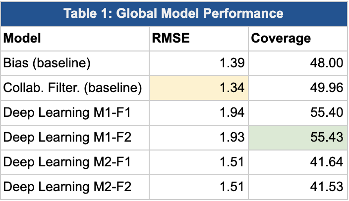
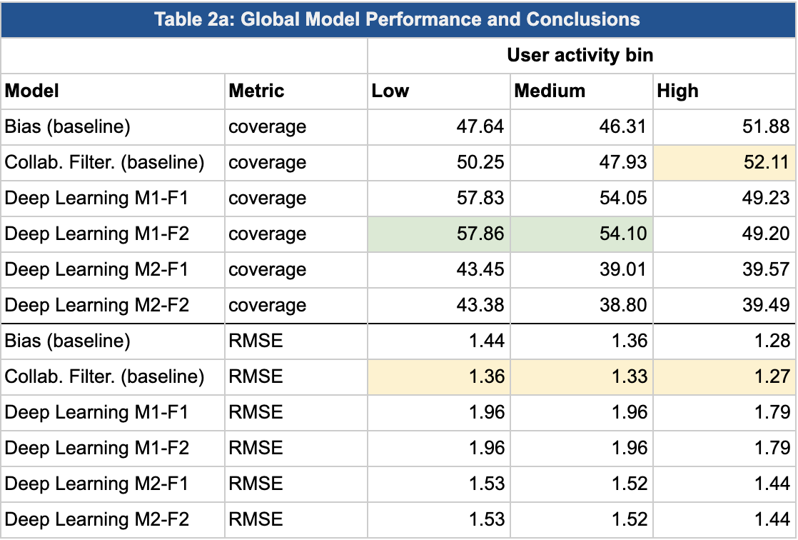
Several patterns become apparent in the table above:
- RMSE:
- Results: On this simple metric, it’s clear that one of our baseline models (Collaborative Filtering, SVD) performs the best. Unfortunately, our Deep Learning models perform worse than the baseline bias model.
- Analysis: We suspect that our Deep Learning models performed worse than our baseline because the architecture of the proposed models are fairly simple and small compared to the industry standard, which require much more data and CPU power.
- Coverage
- Results: Encouragingly, our Deep Learning model performs the best on this dimension. Again, in this context, “coverage” captures the % of predictions for which the predicted rank of the business (for a given user, relative to other businesses) was within 0.25 of the actual rank of the business.
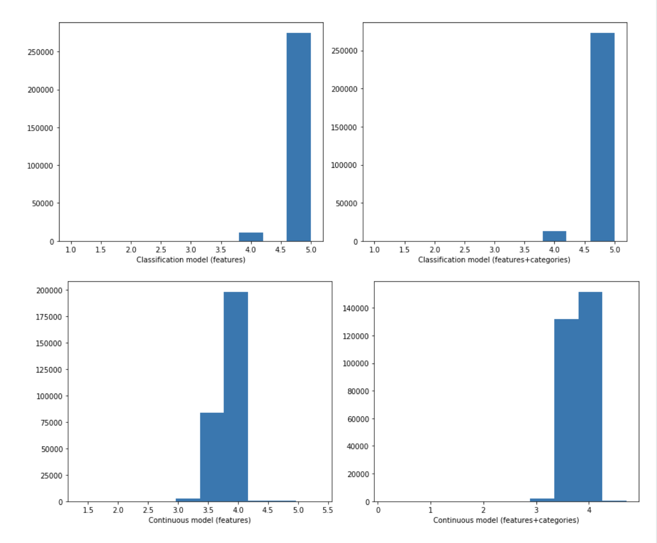
- Analysis: The model that perform best in Coverage is the model of classification approach (i.e. predict a “label” for each review which can take values 1-5) trained with the business and user features plus business categories. Because we treated this as a classification problem, we likely benefited from the fact that our predictions were integer values, and thus when we perform a dense-rank function in computing ranking, our ranking function frequently assigned the same rank to a prediction as the actual rating (which is also an integer value). In fact, we can see in histograms of predictions that this model tend to bias up the predictions values:
Model performance as a function of user-activity and business-popularity:
By user-activity:
By business-popularity:
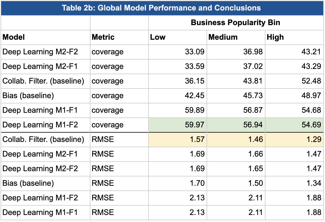
Key Question: Which model has the best performance for low-activity users and for low-popularity businesses? Recall, this was our objective for the project.
Considering that deep learning models are able to learn in a nonlinear way relationships in the data, it may outperform other models in terms of coverage because it doesn’t face problems like cold-start for business that are present in the data. It’s not a surprise that by adding extra information (business categories) the model improves, and we can clearly see that low activity business take advantage of this, because they can consider how other, more popular business with similar categories predict.
The same analysis can be thought for users with low popularity, the model is able to make better predictions for them because it uses the relationships for other similar users.
General Conclusions and Reflection
Our ultimate goal was to identify which recommendation techniques work best for different subsets of the data. In particular, we wanted to understand which models work well for low-activity users and low-popularity businesses; we believe that if we can offer a good product for these users, they are likely to convert into active users.
Encouragingly, our deep learning model had the best performance with respect to coverage for low-activity users. Although we still need to optimize this model by tuning hyper-parameters, we can confidently say that this will at least outperform the baseline. As a result, we can propose a “switching” technique, where we use a deep-learning model early in a user’s lifecycle, and as they become a more active user on the platform, we can switch to collaborative filtering techniques, which are superior for active users.