
Reviews or ratings of products has become almost a mainstream tool nowadays for consumers to support their purchase decision, and retailers know this, specially online retailers. Through online reviews/rating companies can build a trusted reputation on the Internet and influence their revenue. Hence, analysis of reviews and product ratings have become an important source of information about consumer preferences.
Reviews are understood as qualitative - written reviews- or quantitative - ratings - feedback leaved by customers who paid for a product/service. Usually online sites ask for customers to leave a review, after the purchase is done on their website with some sort of system review, mixing a qualitative aspect such as text or a score, number of stars, sad/happy emoji, score bar, etc.
There is certainly a number of factors that influences a review. One could argue that the customer own experience with the product/service is the only catalyst for a good or bad review, but that “experience” can be compromised by much more than just product/service inherent characteristics or brand/company practices. Emotions could play a big role as well as certain demographics, such as sex, age, income, social background and others. The drawback is that companies don’t/can’t collect so much personal information, and reasonably, users won’t give that data either (as easily or for free). Consequently, the majority of literature concerning online reviews revolves around the first and not so much on the latter.
In this context, I thought it would be interesting to study product/service reviews from a perspective of customer’s nationality and explore whether there is a cultural influence given by our country of origin/residence in reviewing products or services, claiming that, generally speaking some cultures can be more inquisitive, while others more laid-back, less-more materialist, have cultural stereotypes among a big number of differences.
One service where a lot of people from different countries converge to is hotels, and thanks to companies for online booking, like Expedia, Trivago, Priceline, Booking, Hotels.com and others, we can search, compare and pick among thousand of hotels. These sites rely heavily on past guest reviews to rank and list hotels for any search the user may do, including features like price, location, amenities, stars and so on. All of these sites have different review systems, but generally, they focus on two components: a written review and a score of some sort. These reviews can also show some user data and are often asked after the guest’s stay has ended.
Having in mind the goal of this analysis, I picked the online site Booking.com. This site displays on every hotel review leaved by a guest its nationality (or country of residence), so it’s a good proxy to explore statistically significant differences. And if so, do people from a common geographic area tend to score lower or higher consistenly? What hotel features do tourists from different places care for more? Do hotels with an international profile tend to get better scores from local or international tourists? These are the types of question I’m looking to answer with the data collected from Booking.com.
Description of the data source
Booking.com has a very nice feature in their review system, not only you can view written reviews in many different languages, but they also display the country of the user that wrote the review. Each hotel’s review has two components: an overall score list of the hotel and its features and the full list of guest reviews, which are breakdown into a written part and an individual score.
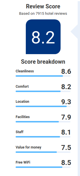

I will focus my analysis in the quantitative part of the review, collecting the overall and individual scores. The overall score is calculated with at least 5 reviews and it’s based on the last 24 months reviews.
The selection of hotels scores data I collected is a subset of hotels in the United States, who receive a variety of tourists from around the world each year. I picked the top 10 most visited cities in United States according to the U.S. Department of Commerce, ITA, National Travel & Tourism Office in 2017.
When you look for a city in the site, it shows you a list of properties which you can sort by a variety of options, no matter what’s the hotel availability:
- Our Top Picks
- Price(lowest first)
- Stars
- Star rating and price
- Distance From Downtown
- Top Reviewed
I chose to stick with the default of the site, which is the “Top Picks” and collect basic data of all the hotels in that list. Afterwards, for each collected hotel, I got the overall and individual scores from the full list of guest scores for all languages. The collection of data was made with a self-coded web scraping script written in Python ad-hoc to this task and was stored in several json files. As the web scraping process was done in two steps, it was natural to come up with two different, but linked, datasets: one for hotels and their basic information along with the overall score, and a second one with the guest’s scores for each hotel. Aditionally, a third python script was needed to scrape the number of stars of each hotel in the site, and was later incorporated into the hotels dataframe.
These files, along with the raw data can be found in my GitHub Repository: Github Repo.
Hotels Dataframe
hotels_df = read_csv("./hotels.csv")
hotels_df = hotels_df %>%
  select(-X1) %>%
  mutate(city = as.factor(city) , reviews= as.factor(reviews))

#add stars feature
stars = read_tsv("./top10us_scrape/unique_hotelstars", col_names = FALSE)
stars = stars %>%
  select(city = X1, hotel_name = X2, hotel_stars = X3) %>%
  mutate(city = as.factor(city), hotel_stars = as.factor(hotel_stars))

hotels = hotels_df %>%
  left_join(stars, by = c("city", "hotel_name"))

#remove some duplicates from the joint
hotels = hotels[!duplicated(hotels$hotel_id),]

sort_hvars = c("hotel_id","hotel_name","hotel_address","city","hotel_stars","review_score","cleanliness","comfort", "location", "services","staff","value_formoney","wifi","reviews")

hotels = hotels[,sort_hvars]

kable(head(hotels[50:100,]))%>%
  kable_styling(full_width = T, font_size = 11.5)%>%
  row_spec(0, bold = T, background = "#BBE9EF")
| hotel_id | hotel_name | hotel_address | city | hotel_stars | review_score | cleanliness | comfort | location | services | staff | value_formoney | wifi | reviews |
|---|---|---|---|---|---|---|---|---|---|---|---|---|---|
| 50 | DoubleTree by Hilton Hotel Los Angeles - Westside | 6161 West Centinela Avenue, Culver City, Los Angeles, CA 90230, United States of America | LosAngeles | 3 | 7.7 | 8.0 | 7.9 | 7.6 | 7.7 | 8.2 | 7.0 | 7.4 | 1 |
| 51 | Doubletree by Hilton Los Angeles Downtown | 120 South Los Angeles Street, Downtown LA, Los Angeles, CA 90012, United States of America | LosAngeles | 4 | 7.7 | 8.2 | 8.0 | 7.7 | 7.7 | 8.2 | 6.8 | 6.2 | 1 |
| 52 | Downtown Condo with Free Parking | W 6th Street and S Bixel Street, Downtown LA, Los Angeles, CA 90017, United States of America | LosAngeles | 0 | NA | NA | NA | NA | NA | NA | NA | NA | 1 |
| 53 | Downtown Cosmopolitan Residences | E 2nd St, S Main St., Downtown LA, Los Angeles, CA 90012, United States of America | LosAngeles | 4 | 8.8 | 9.1 | 9.1 | 8.5 | 9.1 | 8.7 | 8.3 | 8.2 | 1 |
| 54 | Downtown LA Dazzling Apartment | Wilshire Blvd and South Bixel Street, Downtown LA, Los Angeles, CA 90017, United States of America | LosAngeles | NA | 7.6 | 8.2 | 7.5 | 8.0 | 7.1 | 7.7 | 7.3 | 7.5 | 1 |
| 55 | Downtown LA Gorgeous Resort Style Suite | S. Bixel Street and W. 7th Street, Downtown LA, Los Angeles, CA 90017, United States of America | LosAngeles | 0 | 7.3 | 6.9 | 7.5 | 8.1 | 7.0 | 7.5 | 7.1 | 10.0 | 1 |
desc_hotels = data.frame(Variable =sort_hvars,
                         Description = c(
                           "Given hotel ID",
                           "Hotel name",
                           "Hotel address",
                           "City in which the hotel is located",
                           "Stars category of the hotel from 0-5",
                           "Overall score of hotel",
                           "Hotel score on Cleanliness",
                           "Hotel score on Comfort",
                           "Hotel score on Location",
                           "Hotel score on Facilities",
                           "Hotel score on Staff",
                           "Hotel score on Value for Money",
                           "Hotel score on WiFi",
                           "Whether the hotel has or not guest's scores"),
                         Type = c(
                           "Number ranging from 1-6738",
                           "Character",
                           "Character",
                           "Factor with 10 levels",
                           "Factor with 6 levels",
                           "Number with one decimal ranging from 1.0-10.0",
                           "Number with one decimal ranging from 1.0-10.0",
                           "Number with one decimal ranging from 1.0-10.0",
                           "Number with one decimal ranging from 1.0-10.0",
                           "Number with one decimal ranging from 1.0-10.0",
                           "Number with one decimal ranging from 1.0-10.0",
                           "Number with one decimal ranging from 1.0-10.0",
                           "Number with one decimal ranging from 1.0-10.0",
                           "Factor with 2 levels: 0 for no posts"
                         ))


kable(desc_hotels) %>%
  kable_styling(full_width = F, font_size = 13) %>%
  add_header_above(c("", "Hotel Table", "6,738 Observations"), bold = TRUE, align = "c" ) %>%
  column_spec(1, bold = T, border_right = T, background = "#BBE9EF") %>%
  column_spec(2, width = "30em") %>%
  column_spec(3, width = "30em")
| Variable | Description | Type |
|---|---|---|
| hotel_id | Given hotel ID | Number ranging from 1-6738 |
| hotel_name | Hotel name | Character |
| hotel_address | Hotel address | Character |
| city | City in which the hotel is located | Factor with 10 levels |
| hotel_stars | Stars category of the hotel from 0-5 | Factor with 6 levels |
| review_score | Overall score of hotel | Number with one decimal ranging from 1.0-10.0 |
| cleanliness | Hotel score on Cleanliness | Number with one decimal ranging from 1.0-10.0 |
| comfort | Hotel score on Comfort | Number with one decimal ranging from 1.0-10.0 |
| location | Hotel score on Location | Number with one decimal ranging from 1.0-10.0 |
| services | Hotel score on Facilities | Number with one decimal ranging from 1.0-10.0 |
| staff | Hotel score on Staff | Number with one decimal ranging from 1.0-10.0 |
| value_formoney | Hotel score on Value for Money | Number with one decimal ranging from 1.0-10.0 |
| wifi | Hotel score on WiFi | Number with one decimal ranging from 1.0-10.0 |
| reviews | Whether the hotel has or not guest's scores | Factor with 2 levels: 0 for no posts |
Guest Reviews Dataframe
posts = read_csv("./posts_2.csv")
posts = posts %>%
  select(-X1) %>%
  mutate(city = as.factor(city),
         review_country= as.factor(review_country),
         review_date = as.Date(review_date, format= "%B %d,%Y"))

sort_pvars = c("hotel_id","city","review_id","review_score","review_date","review_country", "review_number")

posts = posts[,sort_pvars]

kable(head(posts[50:100,]))%>%
  kable_styling(full_width = T, font_size = 13)%>%
  row_spec(0, bold = T, background = "#BBE9EF")
| hotel_id | city | review_id | review_score | review_date | review_country | review_number |
|---|---|---|---|---|---|---|
| 5 | LosAngeles | 114 | 7.9 | 2018-04-04 | China | 5 |
| 5 | LosAngeles | 115 | 10.0 | 2018-04-03 | Australia | 25 |
| 5 | LosAngeles | 116 | 4.6 | 2018-04-02 | United States of America | 1 |
| 5 | LosAngeles | 117 | 7.9 | 2018-03-30 | United States of America | 2 |
| 5 | LosAngeles | 118 | 8.3 | 2018-03-29 | Belgium | 39 |
| 5 | LosAngeles | 119 | 10.0 | 2018-03-28 | United States of America | 34 |
desc_posts = data.frame(Variable = sort_pvars,
                         Description = c(
                           "Given hotel ID",
                           "City in which the hotel is located",
                           "Given post ID by hotel ID",
                           "Score given by guest to the hotel",
                           "Date that the score was given by guest",
                           "Country reported by guest",
                           "Number of all reviews given up to date from guest in the site"),
                         Type = c(
                           "Number ranging from 1-6738",
                           "Factor with 10 levels",
                           "Number ranging from 1 to number of reviews per hotel (max. 29,596)",
                           "Number with one decimal ranging from 1.0-10.0",
                           "Date with format: YYYY-MM-DD",
                           "Factor with 245 levels",
                           "Number ranging from 1 to number of reviews given by guest (max. 423)"
                         ))

kable(desc_posts) %>%
  kable_styling(full_width = F, font_size = 13) %>%
  add_header_above(c("", "Guest's score Table", "1,712,086 Observations"), bold = TRUE, align = "c" ) %>%
  column_spec(1, bold = T, border_right = T, background = "#BBE9EF") %>%
  column_spec(2, width = "30em") %>%
  column_spec(3, width = "30em")
| Variable | Description | Type |
|---|---|---|
| hotel_id | Given hotel ID | Number ranging from 1-6738 |
| city | City in which the hotel is located | Factor with 10 levels |
| review_id | Given post ID by hotel ID | Number ranging from 1 to number of reviews per hotel (max. 29,596) |
| review_score | Score given by guest to the hotel | Number with one decimal ranging from 1.0-10.0 |
| review_date | Date that the score was given by guest | Date with format: YYYY-MM-DD |
| review_country | Country reported by guest | Factor with 245 levels |
| review_number | Number of all reviews given up to date from guest in the site | Number ranging from 1 to number of reviews given by guest (max. 423) |
Description of data import / cleaning / transformation
The collected data with the python script was dump into json files by city given the structured nature of it. Next, the preprocessing was done by a second python script that parsed the json files into CSV files. These CSV files were read with R into 2 dataframes.
In addition, the variable “review_country” was recoded into a new factor variable “continent” to aggregate the origin of each review into a broader category. This was done in two steps: first, using the R library “countrycode” and second, making some manual changes in continent names creating a small dataframe to replace some continents into more detailed names (like “Canada” coded as “Americas” into “North America”). The resulting variable “continent” is a factor with 8 levels.
library(countrycode)
posts$continent = countrycode(sourcevar = posts$review_country,
                              origin = "country.name",
                              destination = "continent")


americas = data.frame(continent = c("North America","North America","North America", "North America","North America","North America","North America","North America","North America","North America","North America","North America","North America","North America","North America","North America","North America","North America","North America","North America","North America","North America","North America","North America","North America","North America","South America","South America","South America","South America","South America","South America","South America","South America","South America","South America","South America","South America","South America", "Americas", "North America", "North America", "Oceania", "Europe", "Europe", "Asia", "Africa", "Antarctica", "Africa", "South America"),
                      review_country = c("Bermuda","Greenland","Puerto Rico","Antigua and Barbuda","Bahamas","Barbados","Belize","Canada","Costa Rica","Cuba","Dominica","Dominican Republic","El Salvador","Grenada","Guatemala","Haiti","Honduras","Jamaica","Mexico","Nicaragua","Panama","Saint Kitts and Nevis","Saint Lucia","Saint Vincent and the Grenadines","Trinidad and Tobago","United States of America","Argentina","Bolivia","Brazil","Chile","Colombia","Ecuador","Guyana","Paraguay","Peru","Suriname","Uruguay","Venezuela","Falkland Islands (Malvinas)", "Saint Martin", "Saint Barts", "United States Minor Outlying Islands", "Micronesia", "Kosovo", "Crimea", "British Indian Ocean Territory", "Central Africa Republic", "Antarctica", "French Southern Territories",  "South Georgia and the South Sandwich Islands"))
americas$continent = as.character(americas$continent)

posts = posts %>%
  left_join(americas, by="review_country")

posts =  posts %>%
  mutate(continent = as.factor(if_else(is.na(continent.y), continent.x, continent.y))) %>%
  select(-c(continent.x, continent.y))

posts = posts %>%
  mutate(review_continent = as.factor(str_replace(continent, "Americas", "Central America")),
         review_country = as.factor(review_country))%>%
  select(-continent)
Missing values
colSums(is.na(hotels)) %>%
  sort(decreasing=TRUE) %>%
  kable(col.names = "Missing") %>%
  kable_styling(full_width = F, position = "center",bootstrap_options = c("striped", "hover"), font_size = 13) %>%
  column_spec(1, bold = T, border_right = T, background = "#BBE9EF")
| Missing | |
|---|---|
| cleanliness | 3875 |
| comfort | 3875 |
| location | 3875 |
| review_score | 3875 |
| services | 3875 |
| staff | 3875 |
| value_formoney | 3875 |
| wifi | 3875 |
| hotel_stars | 2775 |
| hotel_address | 43 |
| reviews | 0 |
| hotel_name | 0 |
| city | 0 |
| hotel_id | 0 |
tidyhotels <- hotels %>%
    select(-hotel_id) %>%
    gather(key, value, -city) %>%
    mutate(missing = as.factor(ifelse(is.na(value), "yes", "no")), key=as.factor(key),
           value= as.numeric(value))
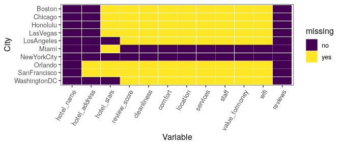
A simple sum of columns let us know the extent of missing value per variable. From the total number of observations, 6,738, we can note that 3,875 values are missing from the score aspects of each hotel. This may be due to lack of guest’s reviews to calculate an overall score explained by a number of reason such that an average experience may not be worth the time to leave a review or the hotel itself doesn’t encourage guests to leave feedback.
We can see a breakdown of these missing values per city in a tile plot. Is easy to see that New York City and Miami are the cities with a more complete profile of data:
ggplot(tidyhotels, aes(x = fct_relevel(key,sort_hvars[-c(1,4)]), y = fct_rev(city), fill = missing)) +
  geom_tile(color = "white") +
  scale_fill_viridis_d() + # discrete scale
  ylab("City") +
  xlab("Variable")+
  theme_bw(12) +
  theme(axis.text.x=element_text(angle=60,hjust=1))
hotels %>%
  filter(!is.na(review_score)) %>%
  mutate(citycount = fct_infreq(city)) %>%
  ggplot(aes(x = fct_rev(citycount))) +
  geom_bar(width = 0.7, color = "black", fill = "thistle") +
  labs(x="City",y= "Number of hotel scores per city without NA's") +
  theme(panel.grid.major.x = element_blank())+
  theme_gray(12)+
  coord_flip()
posts %>%
  filter(!is.na(review_country)) %>%
  mutate(citycount = fct_infreq(city)) %>%
  ggplot(aes(x = fct_rev(citycount))) +
  geom_bar(width = 0.7, color = "black", fill = "thistle") +
  theme(panel.grid.major.x = element_blank())+
  theme_gray(12)+
  scale_y_continuous(breaks =seq(0,700000,100000), labels = scales::comma) +
  xlab("City") +
  ylab("Number of individual scores per city without NA's") +
  coord_flip()
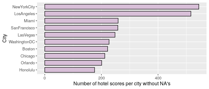
Since the goal of this study is to explore differences within countries reviews, we are going to work only with hotels with complete data (2,863) that accounts for more than 1 million guests reviews in total.
colSums(is.na(posts)) %>%
  sort(decreasing=TRUE)  %>%
  kable(col.names = "Missing") %>%
  kable_styling(full_width = F, position = "center",bootstrap_options = c("striped", "hover"), font_size = 9) %>%
  column_spec(1, bold = T, border_right = T, background = "#BBE9EF")
| Missing | |
|---|---|
| review_country | 1109 |
| review_continent | 1109 |
| review_score | 1 |
| city | 0 |
| hotel_id | 0 |
| review_number | 0 |
| review_date | 0 |
| review_id | 0 |
In fact, we can see from the Reviews Dataframe that only 1 review score is missing and only 1,109 countries out of 1,712,086 observations (0.06%), so I’m going to focus the analysis on this data mainly.
tidystars <- hotels %>%
    select(-hotel_id) %>%
    gather(key, value, -hotel_stars) %>%
    mutate(missing = as.factor(ifelse(is.na(value), "yes", "no")), key=as.factor(key))%>%
    group_by(hotel_stars, key, missing) %>%
    summarise(n = n()) %>%
    ungroup() %>%
    spread(missing,n,fill = 0)
Analysis
Hotel average review scores
First, we analize the hotel-level scores, this is, the average of the scores an hotel gets among all its guests that wrote a review and evaluated it. In other words, each observation correspond to an hotel in the sample.
How does this overall score distributes among hotels?
hotels %>%
  filter(!is.na(review_score)) %>%
  ggplot(aes(review_score))+
    geom_histogram(binwidth = 0.05, color = "black", fill = "#009E73") +
    labs(x = "Hotel overall score") +
    scale_x_continuous(breaks = seq(2,10,0.5)) +
    theme_gray(12)
hotels %>% summarise_at('review_score',list('Min.' = min,
                                            '1st. Quartile' = function(x,...) quantile(x,probs = 0.25,...),
                                            'Median' = median,
                                            'Mean' = mean,
                                            '3rd. Quartile' = function(x,...) quantile(x,probs = 0.75,...),
                                            'Max.'=max), na.rm = T) %>%
  gather(key = "statistic",value = "value",convert = TRUE) %>%
  kable(col.names = c("Statistic","Value"), digits = 2) %>%
  kable_styling(full_width = F, position = "center", font_size = 9) %>%
  column_spec(1, bold = T, border_right = T, background = "#BBE9EF")
| Statistic | Value |
|---|---|
| Min. | 4.00 |
| 1st. Quartile | 7.80 |
| Median | 8.40 |
| Mean | 8.21 |
| 3rd. Quartile | 8.80 |
| Max. | 10.00 |
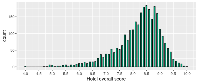
The distribution of hotel overall scores are left-skewed, with high concentration on the high portion of the scale, considering the scores range from 1 to 10. The hotel with the lowest score has a rating of 4.0, whereas 50% of hotels have a score of 8.40 or higher.
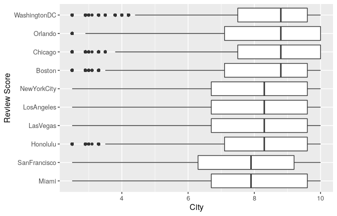
How do this overall score distributes by city?
meds = hotels %>%
  select(city, review_score) %>%
  group_by(city) %>%
  summarise(med = median(review_score, na.rm = TRUE))

ggplot(hotels, aes(x=city, y=review_score)) +
  geom_boxplot()+
  scale_x_discrete(limits=meds$city[order(meds$med)]) +
  coord_flip()+
  labs(y="Hotel overall score",x="City")+
  theme_gray(12)

The distribution of hotel overall scores are dependent on the city. When plotting boxplots of hotel score per city, data seems to suggest that hotels in more expensive cities such as San Francisco and Honolulu tend to have lower scores than others such as Chicago or Orlando, but this is a just a general perception.
Now we can look the breakdown of this overall score in its different categories, do they distribute differently?
tidyhotels %>%
  filter(!is.na(value)) %>%
  filter(!(key %in% c("hotel_name", "hotel_address", "hotel_stars", "reviews"))) %>%
  ggplot(aes(value)) +
    geom_histogram(binwidth = 0.05, fill = "#009E73") +
    xlab("Hotel overall score")+
    facet_wrap(~key, ncol=2) +
    theme_gray(12)
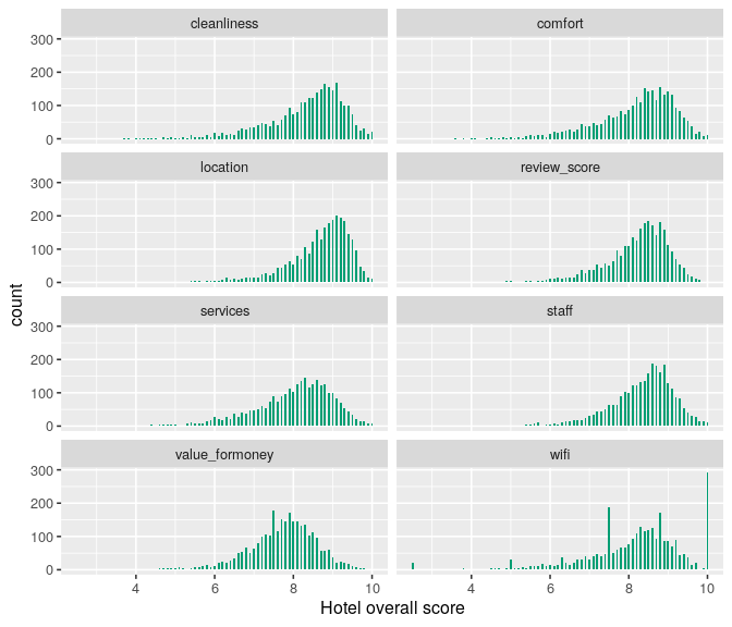
A similar pattern can be shown when disaggregating the hotel overall score into the different features the website allows guests to evaluate the hotels. Guests tend to provide lower scores to value, while providing higher scores to location. Interestingly, there is a high concentration of hotels that obtain a perfect score in the Wi-Fi dimension.
What do we expect if we plot the hotel’s overall score by number of stars?
hotels %>%
  filter(!is.na(review_score) & !is.na(hotel_stars)) %>%
  filter(hotel_stars !=0) %>%
  ggplot(aes(fct_reorder(hotel_stars, review_score, median), review_score)) +
  geom_boxplot() +
  coord_flip() +
  xlab("Hotel Stars")+
  ylab("Hotel overall score")+
  theme_gray(12)
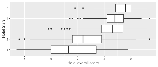
One may expect that hotel’s overall scores reflect to some degree the quality of an hotel. At the same time, hotels are categorized by the website on the attribute “stars”, from 1 (lowest) to 5 (highest), which aims to reveal the amenities and level of service expected from the hotel. The data shows a strong relationship between the hotel overall score, provided by guests, and the number of stars that the hotel has. Interestingly, high stars hotels are distributed only in the higher portion of the scale (most hotels of 4 or more stars have a score higher than 7); whereas hotels with 1 or 2 stars not only have lower scores in average, but also are distributed over a wider range.
Individual guest’s review scores
Now, let’s analize the individual scores provided by guests. In these analysis each observation correponds to one review provided by a guest to an hotel.
Distribution of guest’s scores:
ggplot(posts, aes(review_score))+
  geom_histogram(binwidth = 0.1, color = "black", fill = "#009E73") +
  xlab("Review Score")+
  scale_y_continuous(labels = scales::comma)+
  theme_gray(12)
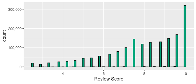
Here we see an interesting and somewhat odd distribution due to some gaps between certain values of the score that the guests give to an hotel. If we look closer, there is indeed values that simply doesn’t happen, but also there is an unexpected behaviour in the amount of values for integer scores: 3, 4, 5, 6, 7, 8 and 9. For review type of values one would expect that people tend to give integer scores or half scores (i.e. 5.5, 8.5, 9.5) but not so much in between, like 9.1 or 2.4. The most pausible explanation for these results resides in the review system of Booking.com, where they present to guests the option to give from 1 to 4 smiley faces for each category and then taking the average of reviewed items (as mentioned in the introduction). With this system, you can easily get the distribution of scores we are observing since each category can get a score in [0, 2.5, 5, 7.5, 10] only, so for example, if you rank 5 with 3 faces and 1 with 1 you’ll get a score of ~6.7. This is why we get a higuer amount of scores with a decimal point rather than integer ones.
Now, let’s break down the guest’s score by city:
pmeds = posts %>%
  select(city, review_score) %>%
  group_by(city) %>%
  summarise(med = median(review_score, na.rm = TRUE))

ggplot(posts, aes(x=city, y=review_score)) +
  geom_boxplot()+
  scale_x_discrete(limits=pmeds$city[order(pmeds$med)]) +
  coord_flip()+
  labs(x="Review Score",y="City")+
  theme_gray(12)
Compared to the distribution of hotel scores by cities, when analyzing individuals’ scores, we can observe how scores are more widely distributed, and mean differences between cities become smaller compared to differences in hotel-level scores.
Country differences in guest’s review scores
In the following, I’ll explore if there’s evidence of differences accross countries for the individual guest’s review scores.
n1000 = posts %>%
  select(review_country) %>%
  count(review_country)%>% filter(n>1000)

posts %>%
  select(review_country, review_score, review_continent) %>%
  filter(!is.na(review_country)) %>%
  group_by(review_country) %>%
  summarise(med = mean(review_score, na.rm = TRUE), sd = sd(review_score, na.rm = TRUE),n = sum(!is.na(review_score)))  %>%
  mutate(lb = med -sd/sqrt(n), ub = med +sd/sqrt(n)) %>%
  filter(review_country %in% n1000$review_country) %>%
  ggplot(aes(med, reorder(review_country,med))) +
  geom_point(color="#883A8B") +
  geom_segment(aes(y = reorder(review_country,med),x = lb,xend = ub,yend = reorder(review_country,med)),color = "#883A8B") +
  ylab("Country") +
  xlab("Guest's review scores mean with standard error") +
  labs(title="Mean of guest review score for countries\nwith more than 1,000 reviews")+
  theme_bw(12) +
   theme(axis.text.y = element_text(size = rel(.75)),
    	axis.ticks.y = element_blank(),
        axis.title.x = element_text(size = rel(.75)),
        panel.grid.major.x = element_blank(),
        panel.grid.major.y = element_line(size = 0.7),
        panel.grid.minor.x = element_blank())
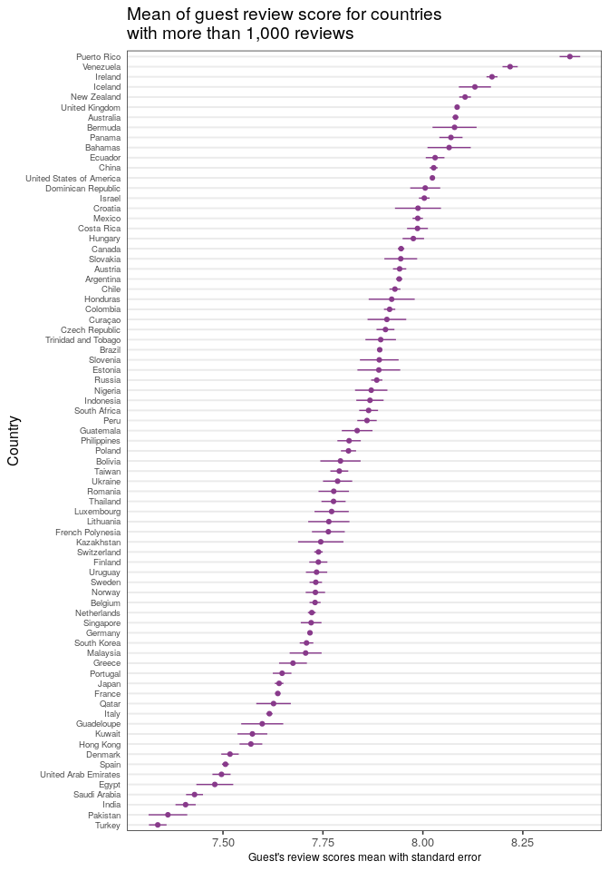
The graph shows the different scores means by country and given the high number of reviews per country (filter on more than 1,000) there’s a good approximation for the mean standard error. The bar error help us noting that as the mean goes down by country its error bar is not overlapping within different sections of the scale, for example, if we compare the countries with means around 7.5 and 7.75 there’s practically no overlapping with the ones in the range 7.75 and 8 (i.e. with a 0.5 difference in score).
This plot is probably the most revealing one, as it let us see and compare across countries.
Now, let’s check the guest’s review score standard deviation by country:
posts %>%
  select(review_country, review_score) %>%
  filter(!is.na(review_country)) %>%
  group_by(review_country) %>%
  summarise(sdc = sd(review_score, na.rm = TRUE))  %>%
  filter(review_country %in% n1000$review_country) %>%
  ggplot(aes(sdc, reorder(review_country, sdc))) +
  geom_point(color="#FF8011") +
  ylab("Country") +
  xlab("Standard Deviation of review score") +
  labs(title="Standard Deviation of guest review score\nfor countries with more than 1,000 reviews")+
  theme_bw(12) +
   theme(axis.text.y = element_text(size = rel(.75)),
    	axis.ticks.y = element_blank(),
        axis.title.x = element_text(size = rel(.75)),
        panel.grid.major.x = element_blank(),
        panel.grid.major.y = element_line(size = 0.7),
        panel.grid.minor.x = element_blank())
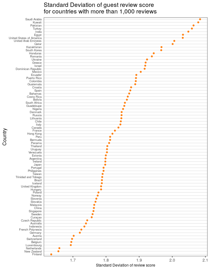
Here we see evidence that the variation on how people review hotels may indeed be different accross countries on this sample. A closer look at the plot show us that, for example, for countries like Saudi Arabia, Kuwait, Pakistan, Turkey, India, Egypt, United Arab Emirates and Qatar, to name a few, there are travelers who rate very high and travellers that doesn’t seem to enjoy their stay very much. In contrast, countries like Germany, Austria, Switzerland, Belgium, Luxembourg, The Netherlands and Finland, seem to review in a very similar way.
Not considering the United States, the pattern is very intriguing for this sample: countries from very close regions of the world (in this case the Middle East and Northern Europe) tend to review with a similar criterion.
Next, I am curious to see if the mean score by country changes with the number of stars of a hotel. Let’s explore the mean score and its error for hotels in the category of 4 or 5 stars and in the category of 2 or 3:
n5000 = posts %>%
  select(review_country) %>%
  count(review_country)%>% filter(n>5000)

post_filterstars = posts %>%
  select(review_country, review_score, hotel_id) %>%
  filter(!is.na(review_country)) %>%
  left_join(hotels, by="hotel_id") %>%
  select(review_country, review_score.x, hotel_stars) %>%
  filter(!is.na(hotel_stars)) %>%
  filter(hotel_stars != 0) %>%
  group_by(hotel_stars, review_country) %>%
  summarise(mean = mean(review_score.x, na.rm = TRUE), sd = sd(review_score.x, na.rm = TRUE),n = sum(!is.na(review_score.x)))  %>%
  mutate(lb = mean -sd/sqrt(n), ub = mean +sd/sqrt(n))
s1 =  post_filterstars %>%
      filter((review_country %in% n5000$review_country) & (hotel_stars==1 | hotel_stars==2)) %>%
      ggplot(aes(mean, reorder(review_country,mean), color=hotel_stars)) +
      geom_point() +
      labs(x="Review Score mean", y="Country",color = "Hotel stars", title="Guest's review score mean by country for \n1 and 2 star hotels with more than 5,000 reviews") +
      geom_segment(aes(y = reorder(review_country,mean),x = lb,xend = ub,yend = reorder(review_country,mean),color = hotel_stars)) +
      scale_x_continuous(breaks = seq(5,10,0.5),limits = c(4.5,9)) +
      theme_bw(12) +
       theme(axis.text.y = element_text(size = rel(.75)),
        	axis.ticks.y = element_blank(),
            axis.title.x = element_text(size = rel(.75)),
            panel.grid.major.x = element_blank(),
            panel.grid.major.y = element_line(size = 0.7),
            panel.grid.minor.x = element_blank())

s2 = post_filterstars %>%
      filter((review_country %in% n5000$review_country) & (hotel_stars==5 | hotel_stars==4)) %>%
      ggplot(aes(mean, reorder(review_country,mean), color=hotel_stars)) +
      geom_point() +
      labs(x="Review Score mean", y="Country",color = "Hotel stars", title="Guest's review score mean by country for \n4 and 5 star hotels with more than 5,000 reviews") +
      scale_x_continuous(breaks = seq(5,10,0.5),limits = c(4.5,9)) +
      geom_segment(aes(y = reorder(review_country,mean),x = lb,xend = ub,yend = reorder(review_country,mean),color = hotel_stars)) +
      theme_bw(12) +
       theme(axis.text.y = element_text(size = rel(.75)),
        	axis.ticks.y = element_blank(),
            axis.title.x = element_text(size = rel(.75)),
            panel.grid.major.x = element_blank(),
            panel.grid.major.y = element_line(size = 0.7),
            panel.grid.minor.x = element_blank())


gridExtra::grid.arrange(s1, s2, ncol=2)
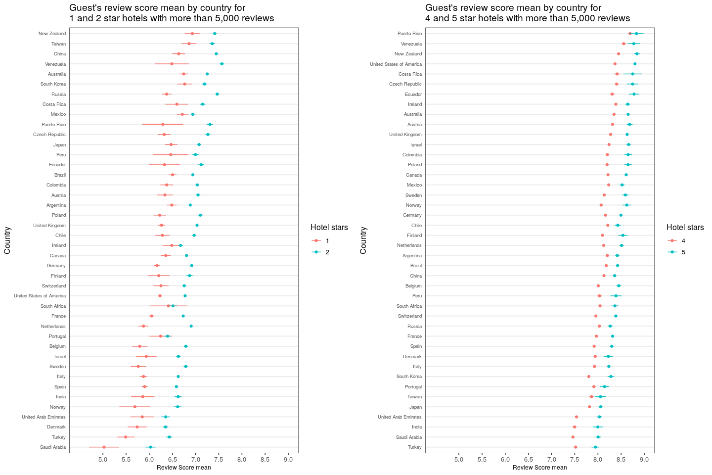
Convincingly, even if we control by the number of stars a hotel is categorized into, the patterns of differences by countries still remain true in this sample. One can notice this by looking at the first and last country in each plot and observe that the mean is consistenly different and there’s almost no overlapping considering the error when splitting by stars.
Taking advantage of the created variable “continent” I am interested to find if the differences observed are replicable in broader regions of procedence, such as a continent.
posts %>%
  select( review_score, review_continent) %>%
  filter(!is.na(review_continent)& review_continent!="Antarctica") %>%
  ggplot(aes(x=fct_reorder(review_continent, review_score, median), y=review_score)) +
  geom_boxplot() +
  coord_flip()+
  xlab("Continent")+
  ylab("Review Score")+
  theme_gray(12)
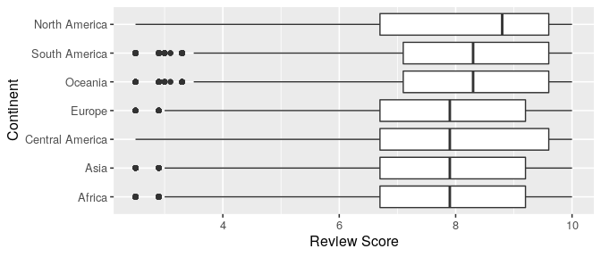
By aggregating where the reviews come from in a broader scale, such as continents, we observe that the pattern is not so clear anymore. All continents seems to have a very similar distribution with some minor differences, being countries from North America the ones with a higher median of review score. But, certainly, all continents have the same range of data and similar quartiles and medians scores.
posts %>%
  select( review_score, review_continent) %>%
  filter(!is.na(review_continent) & review_continent!="Antarctica") %>%
  ggplot(aes(review_score, fct_reorder(review_continent, review_score, median))) +
  geom_density_ridges(scale=2, fill = "lightblue") +
  scale_x_continuous(breaks = seq(2,10,1)) +
  theme_gray(12)+
  labs(x = "Review Score", y="Continent")
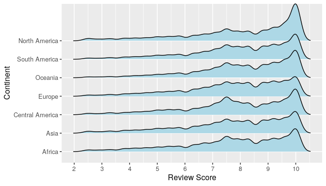
The ridge line plot seems to reveal that distributions of scores for all continents could have a second, lower, median, coming maybe from a bimodal distribution.
top3continent = posts %>%
  select(city, review_continent) %>%
  filter(!is.na(review_continent) & review_continent!="Antarctica") %>%
  group_by(city) %>%
  count(review_continent) %>%
  mutate(N=sum(n)) %>%
  arrange(city, desc(n)) %>%
  ungroup() %>%
  mutate(freq = n/N)

ggplot(top3continent, aes(x=review_continent, y=freq, group=city)) +
  geom_col(fill = "#009E73") +
  facet_wrap(~city, nrow=5) +
  scale_y_continuous(labels = scales::percent)+
  labs(y="Percentage of reviews by city", x="Continent")+
  coord_flip()+
  theme_gray(12)
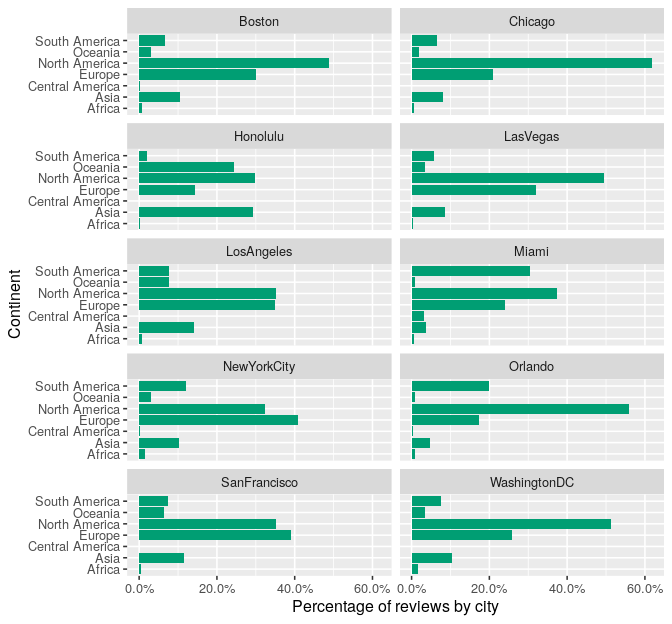
This plot reveals that if we facet the number of reviews per continent by cities we see some differences on the proportion of tourists from different continents.
Worth noting that San Francisco and New York City are the only cities that get more European tourists than local tourists, in comparison to all other cities, in this site in particular. The other interesting fact to observe is how Asian tourists are low on proportion in all cities but Honolulu, where the proportion is almost the same as the North American travellers. Equally interesting, but not surprising, is the porportion of South Americans tourists visiting (and reviewing) Miami and Orlando in contrast with other cities.
Conclusions
Even though non of the patterns and findings of this exploratory analysis are causal effects, there were very interestings correlations going on.
I found some not obvious, but expected results such as:
- The highest number of reviews in every city of the study come from local travelers
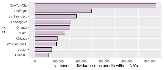
- The cities with the highest number of reviews are New York City and Los Angeles, not surprinsingly, the biggest cities in the sample
- For individual guests scores, New York City is the one with the biggest proportion of reviews
Other findings regarding scores distributions:
- Almost all scores in the study are left skewed with medians around a score of 8.0
- The overall hotel score distributions are susceptible to differences by cities
- The overall hotel score distributions are susceptible to the number of stars of the hotel, as expected, more luxury hotels tend to have better scores than more regular ones. Here, the services, staff and quality seem to accomplish their purpose
- The way in which a site decides to design its review system is going to have a huge impact in the way reviews are distributed. It was possible to unveiled an odd behavior of scores due to the structure of the score guests can give on Booking.com
The main and most meaningful finding of this analysis was the fact that the sample did present some differences in guest’s scores for hotels in US cities when looking at the country tourists come from. When filtering countries with more than 1,000 reviews, there’s room to think that differences are most decisevely. This fact is replicated when looking at the variance of scores per country. The sample suggests there are distinctive world regions when considering how much heterogeneity there is in scores people give to their stays. This alone is particularly intriguing and deserves a closer look, and may be hepful for companies to think on a more customizable experience.
In next steps, I would consider the addition of new variables to control the review score per country and study whereas or not the differences persist. These variables could be exogenous such as demographics of cities, whether the guests are often travelers or not, what type of trip is the visit (business, leisure, etc.). But there’s, categorically, more questions to be asked.