
With the recent changes to Google API, the ggmap library is no longer totally free to use (you can read more about it here). I was wondering what other alternatives there are in R to make not only beautiful, but useful maps with all the ggplot machinery at your hands.
Although, the new API charges may not be pricey for moderate use, if you use ggmap sparingly, like me, the service might just not be worthy. So, what other R resources are out there?
-
The old but trusted shape file
-
ggmapwith Open Source maps
Let’s get some datasets with location data and make some maps!
Load libraries
library(ggplot2)
library(sf)
library(ggmap)
library(tidyr)
library(dplyr)
Load and Read Datasets
I’ve chosen to plot the recently added open datasets of the state of Vermont, particularly of its most populous city, Burlington. You can find these and other interesting datasets in the city’s new portal of Open Data here.
I picked the “Tree Database” which contains all trees currently managed by the city, and the schools (public and private) data set along with the childcare sites around the city.
#trees dataset
trees = read.csv("planting-sites.csv", sep=";")
#public schools dataset
schools = read.csv("us-public-schools.csv", sep=";")
#private schools dataset
schools_private = read.csv("us-private-schools.csv", sep=";")
#child care dataset
childcare = read.csv("child-care-locations.csv", sep = ";")
Preprocess the data
We need to get the data ready before anything else, so here I do some processing of the data, specifically:
- Split the
Geo.Pointcolumn into two separates columns of latitude and longitude for each data set and change its type to numeric variables. - Filter schools for the city of Burlington.
- We will use the column
Enrollmentof schools to plot schools by size
trees = trees %>%
  separate(Geo.Point, c("lat","long"), ",")

trees = trees %>%
  mutate(lat = as.numeric(lat),
         long = as.numeric(long))


bt_schools = schools %>%
  separate(Geo.Point, c("lat","long"), ",")

bt_schools = bt_schools %>%
  mutate(lat = as.numeric(lat),
         long = as.numeric(long),
         Enrollment = as.numeric(Enrollment))

#filter schools only for burlington with greater than zero enrollment
bt_schools = bt_schools %>%
  filter(City %in% c("BURLINGTON") & Enrollment>0)


bt_schools_private = schools_private %>%
  separate(Geo.Point, c("lat","long"), ",")

bt_schools_private = bt_schools_private %>%
  rename(Enrollment = ENROLLMENT ) %>%
  mutate(lat = as.numeric(lat),
         long = as.numeric(long),
         Enrollment = as.numeric(Enrollment))

#filter private schools only for burlington
bt_schools_private = bt_schools_private %>%
  filter(CITY %in% c("BURLINGTON") & Enrollment>0)


childcare = childcare %>%
  separate(geo_point, c("lat","long"), ",")

childcare = childcare %>%
  mutate(lat = as.numeric(lat),
         long = as.numeric(long)) %>%
  filter(lat>44)
Subsetting
Lastly, we are going to modify the dataframes, by selecting the relevant columns and creating two new ones: type and point_size to differentiate points when we plot them.
sb_trees = trees %>%
  select(long, lat) %>%
  mutate(type = "Trees",
         point_size = "small")

sb_schools = bt_schools %>%
  select(long,lat, Enrollment) %>%
  mutate(type = "Public schools",
         point_size = Enrollment)

sb_schools_priv = bt_schools_private %>%
  select(long,lat, Enrollment) %>%
  mutate(type = "Private schools",
         point_size = Enrollment)

sb_childcare = childcare %>%
  select(long,lat) %>%
  mutate(type = "Child Care",
         point_size = "small")
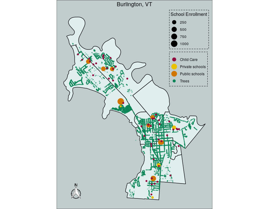
Option 1: get your shape file
To make this option works, we first need to get our hands on a shape file of the location we are trying to map. I found this to be fairly easy, specially for major cities. There are a bunch of shape files available online, like this US states map. Here, you need to decide what type of location granularity you want to display your data on, it can be from a broader perspective such as states, or a very fine division such as districts or counties. So you need to look for your shape file accordingly.
I got Burlington city wards and districts shape file from the same Open Data Portal of the city.
Get Shape file
From here on, we’ll make use of the library sf (special features) to work easily with spatial data but maintaining the same logic of layers in a plot when working with ggplot.
Once you have your shape file, we are going to read it using the st_read function from sf library. It will display the geometry information of the shape file.
bt_shape = st_read("./city-wards-and-districts/city-wards-and-districts.shp")
## Reading layer `city-wards-and-districts' from data source `/home/jaraya/Documents/datasets/burlington_trees/city-wards-and-districts/city-wards-and-districts.shp' using driver `ESRI Shapefile'
## Simple feature collection with 8 features and 4 fields
## geometry type:  POLYGON
## dimension:      XY
## bbox:           xmin: -73.27776 ymin: 44.44592 xmax: -73.1758 ymax: 44.53994
## CRS:            4326
Create Sf datasets
Now, we need to transform our dataframes to an sf object. What this basically do is take the columns with coordinates, such as longitude and latitude, and convert them into a geometry column, we’ll use the st_as_sf function.
trees_sf = st_as_sf(sb_trees, coords = c("long","lat"), remove = FALSE, crs = 4326, agr ="constant")

bt_schools_sf = st_as_sf(sb_schools, coords = c("long","lat"), remove = FALSE, crs = 4326, agr ="constant")

bt_schools_priv_sf = st_as_sf(sb_schools_priv, coords = c("long","lat"), remove = FALSE, crs = 4326, agr ="constant")

childcare_sf = st_as_sf(sb_childcare, coords = c("long","lat"), remove = FALSE, crs = 4326, agr ="constant")
Let’s plot!
If you are familiar with ggplot, this is very straightforward, but instead of the usual ggplot layers such as geom_point, we’ll use the function geom_sf to display our data based on location.
I first started adding the shape file layer to then add the trees, schools and childcare points as we need to, with the same function. With a tweak in colors, sizes and other options, we can get a simple yet informative map fairly quickly:
ggplot() +
  geom_sf(data = bt_shape, size = 0.5, color = "black", fill = "azure2") +
  geom_sf(data = trees_sf, aes(color = type, alpha = type),
          size = 0.5, show.legend = "point") +
  geom_sf(data = bt_schools_sf, aes(color = type, size = point_size, alpha = type),
          stroke=1, show.legend = "point") +
  geom_sf(data = bt_schools_priv_sf, aes(color = type, size = point_size, alpha = type),
          stroke=1, show.legend = "point") +
  geom_sf(data = childcare_sf, aes(color = type, alpha = type),
          size = 1.5, show.legend = "point") +
  scale_color_manual(name = "", values = c("#900c3f","#eac100","#cf7500","#0b8457")) + #childcare, public, private, trees
  scale_alpha_manual(guide = 'none', values = c(1, 1, 1,0.3)) +
  scale_size(name = "School Enrollment") +
  ggtitle("Burlington, VT") +
  guides(color = guide_legend(title = NULL, override.aes = list(size = c(3,5,5,2)))) +
  theme_void() +
  theme(plot.background = element_rect(fill = "azure3"),
        legend.position = c(0.85, 0.8),
        plot.title = element_text(hjust = 0.5),
        legend.background = element_rect(fill = "azure3", color = "black", linetype = "dashed"),
        legend.margin = margin(4, 4, 4, 3, "pt")) +
  coord_sf() +
  ggsn::north(trees_sf, location = "bottomleft")
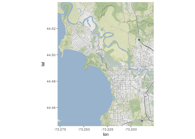
Option 2: Open source maps
Here, things are a little bit different. First, we’ll get an Open Source map from either StatenMaps or OpenStreetMaps, using the same function for Google maps, get_map from the ggmap library.
Here is when it can get a little bit hard, you need to know the limits of the map you are trying to fetch. Think of a square, basically the x and y coordinates of your location such as xmin = left, xmax = right, ymin = bottom and ymax = top. I knew these values from just looking at my shape file, so that’s one very easy way to do it, other way could be to head to Google maps and look for the place you are trying to map and get the coordinates approximately. Then, you can calibrate as you see the map you are getting.
bbox = c(left = -73.27776, bottom = 44.44592, right = -73.1758, top = 44.53994)

p = get_map(bbox, zoom=14, source = "osm", maptype = "roadmap")

ggmap(p)
Once you get the right map, just pass it as input to the ggmap function and then create your map with the ggplot machinery. We are using the same points as before, but using the geom_point function to add them as layers to the ggmap object.
ggmap(p) +
  geom_point(data = sb_trees, aes(long, lat, color = type, alpha = type), size= 0.5) +
  geom_point(data = sb_schools, aes(long, lat, color = type, alpha = type, size = point_size)) +
  geom_point(data = sb_schools_priv, aes(long, lat, color = type, alpha = type, size = point_size)) +
  geom_point(data = sb_childcare, aes(long, lat, color = type, alpha = type), size= 1.5) +
  scale_color_manual(name = "", values = c("#900c3f","#eac100","#cf7500","#0b8457")) + #childcare, public, private, trees
  scale_alpha_manual(guide = 'none', values = c(1, 1, 1, 0.2)) +
  scale_size(name = "School Enrollment") +
  ggtitle("Burlington, VT") +
  guides(color = guide_legend(title = NULL, override.aes = list(size = c(3,5,5,2)))) +
  theme_void() +
  theme(plot.background = element_rect(fill = "azure3"),
        legend.position = c(0.85, 0.75),
        legend.background = element_rect(fill = "azure3", color = "black", linetype = "dashed"),
        legend.margin = margin(4, 4, 4, 3, "pt"),
        plot.title = element_text(hjust = 0.5),
        plot.margin = margin(2, 2, 2, 2, "pt")) +
  coord_quickmap() +
  ggsn::north(sb_trees, location = "bottomleft")
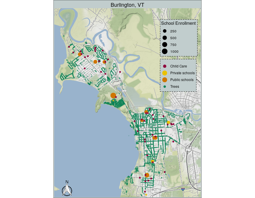
and voilà!
Finally, a nice thing to add to any map are the classic scale symbols, such as north and kms/miles scale. You can do this with the ggsn library with the north method. A warning when you use this with ggmap objects, you would need to add a coordinate system to the object for it to know where it should be placed. I found that coord_quickmap does the trick.